基于腾讯 ACM MM 的视频盲水印

This is the answer of ChatGPT:

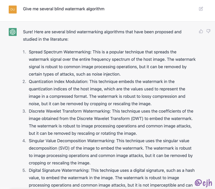
Based on my cognition, this is an exact answer. It digested several main feasible directions of the blind watermarks. Including SVD / DWT / DCT.

Reference

There have many related papers, but what I most referenced is this:

• Adaptive Region Selection Blind Video Watermark (Tencent)
• blind_watermark (Github Open Source)

Github blind_watermark Explain

Before optimizing the current method, we need to know where the bottleneck is. The traditional blind-watermark summary can reference in this paper.

The essential principle is the competition relationship among imperceptibility, robustness, and algorithm efficiency(especially in video watermark).

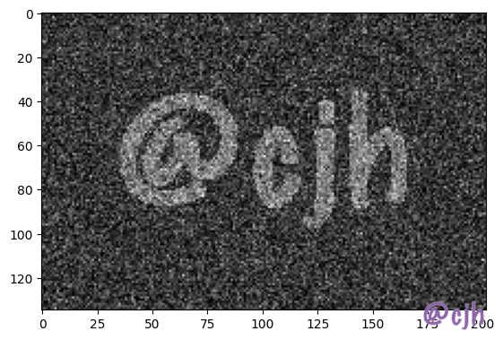
For the Github blind_watermark implementation, which split the image into 8x8 blocks first, then uses the DWT, and DCT respectively. Then shuffles the DCT coefficients to achieve the watermark encryption. Finally, embed the watermark bit into the biggest singular value of SVD coefficients using the quantization method. For extraction, which just is inversed operates on embedding. After that, using k-means to cluster to predict whether the current block bit is 0 or 1.

This method is very robust for JPEG compression, since it uses the same block size as JPEG compression. Under my testing, whose BER(Bit Error Rate) is under 10% while JPEG quality=40.

But in the other hand, this method is very fragile for geometry attacks. can not undertake more than 1-degree rotation. Since any geometry attack is all gonna break the JPEG block sequence.

About imperceptibly, this method is also not good, the Quantization bit embedding process will incur JPEG block effect.

Adaptive Region Selection Method

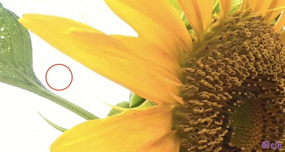
Tencent method first uses the OpenCV ORB algorithm and SVD coefficient weight to select robust 8x8 blocks. After DWT and DCT, embed the watermark bit into the blue channel by the Channel Reference algorithm. This embedding method is more fragile compared to the Quantization method but has good imperceptibility for human eyes, and good robustness for geometry attacks.

But under my testing, for a single image, it only can embed around 1 bit safely, otherwise, the order of ORB feature points will be lost.

Below shows a part of a high-resolution image embedded watermark using channel reference, you can see the light yellow block in the white region where the pixel value is around 0xffffff.

Video Watermark Implementation

Using Hamming 7,4 encoding method to correct the bit error.

Finally efficiency: around 20ms/frame under 1920x1080p 30fps testing video, the processing speed(including watermark bit embedding and HEVC encoding) is 25ms/frame on my MacOS 2020 M1 chip, using the hevc_videotoolbox hardware encoding under FFmpeg.

The average PSNR is 46, for the average bitrate lower than 3M, the watermark will be lost. For the adaptive bit rate stream, the watermark is easier to lose.

For performance, the main cost is splitting / DWT / SVD, for about 17ms, the ORB cost is 3 ms. Thanks to the Numpy FORTRAN matrix optimization, I can use python as fast as C.

Lossless image scale

using linear interpolation and DWT can scale and rescale image lossless, only need to record the scale coefficients.

无损缩小

对于无损缩小有好几种实现方法。这里使用两点 linear scale。首先读取原图像，并对其差分，得到每两点之间的斜率，将离散图像转换为连续的分段函数。然后再根据目标大小对离散图像进行插值。最终返回的是目标图像和原图像的差分。

对目标图像的任何操作都相当于对 $y=kx+b$ 中的 bias 部分进行操作。

无损恢复

已知缩小后的函数是在原连续分段函数上的采样，则可以先根据原图像大小，将缩小后的函数 scale 到原函数大小的区间。

此时对于原图两点之间必须至少知道一点，则可以恢复原图。

具体应用

ORB获取图像特征后，对特征区域进行无损缩放到 8x8 大小，然后进行水印嵌入。

这样得到的特征具有尺度不变性，无论图像的缩放倍数是多少，只要检测到的特征点一致，那么最终缩放得到的8x8大小矩阵就是一样的。

但是当特征区域缩小再放大后将会产生图像质量损失。这种 scale 算法就是用来消除这种质量损失的。

一般需要配合 haar 小波变换，因为如果是一次性 scale 到指定大小然后进行嵌入，该算法将导致较大的图像失真，效果不如 haar

import matplotlib.pyplot as plt
import numpy as np

# 1-D lossless linear scale
def scale(ar: np.ndarray, size: int, axis=-1) -> [np.ndarray, np.ndarray]:
    diff = np.diff(ar, axis=axis)
    p = np.linspace(0, ar.shape[axis], size, endpoint=False)
    left_p = p.astype(int)
    delta_x = p - left_p
    delta_y = diff[left_p] * delta_x
    ret = ar[left_p] + delta_y

    return ret, diff

def inverse_scale(x: np.ndarray, diff: np.ndarray) -> np.ndarray:
    size = diff.size + 1
    assert x.size < size, 'current size must less than original size'
    p = np.linspace(0, size, x.size, endpoint=False)   # restore sample points
    left_p = p.astype(int)
    related_diff = (diff[left_p])
    left, right = x - (p-left_p) * related_diff, x + (1-p+left_p) * related_diff
    ret = np.zeros(size)
    ret[left_p] = left
    ret[left_p+1] = right

    # restore only when scale greater than 2x
    restored_idx = np.unique(np.hstack((left_p, left_p+1)))
    indices_will_restore_count = 1
    remains = None
    while indices_will_restore_count:
        remains = np.setdiff1d(np.arange(size), restored_idx, assume_unique=True)
        indices_will_restore = remains[:-1][np.diff(remains) > 1]
        ret[indices_will_restore] = ret[indices_will_restore+1] - diff[indices_will_restore]

        restored_idx = np.hstack((restored_idx, indices_will_restore))
        indices_will_restore_count = indices_will_restore.size
    for i in remains:
        ret[i] = ret[i-1] + diff[i-1]
    return ret

t = np.linspace(-np.pi, np.pi, 1024)
ar = np.sin(t) + 3*np.cos(3*t)
dst, diff = scale(ar, 10)

dst[5] *= 2

plt.plot(t, ar)
ar_restore = inverse_scale(dst, diff)
# ar_restore = inverse_scale(ar_restore, diff)
plt.plot(t, ar_restore);

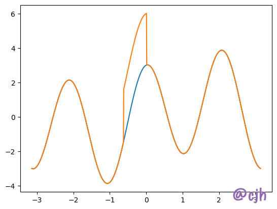
从上图可以看见，对于 scale 以后的信号进行操作，相当于对未 scale 的信号进行相同比例的操作。由此对信号的操作具有尺度不变性。 这里的问题在于，当信号进行压缩时，类似的尖峰脉冲信号很容易就会被抹平。 原因是对于信号的拟合被限制在两点之间，当连续的五个点中的第三个点发生变化时，只会影响到旁边的两个点，而其他点不会有任何影响。

如何对 scale 以后的信号进行操作，将尖峰的信号变化隐藏在领域宽度为 l 的区间内？ 可以使用加权线性插值。将普通的有两个点参与的差分拓展到有 N 个点参与的加权差分，通过最小二乘法求近似解，对于离中心点越远的差分点取越低的权重。

这种方法是可以写出来的，但有两个前提必须先搞清楚： 1 尖峰脉冲在图像压缩中具体的鲁棒性 2 二维 scale / iscale 函数

对于一维插值在二维上的拓展可以参考MR-SVD 中的做法

简单说下 MR-SVD，就是通过坐标奇偶将一维信号转为二维信号，然后通过 PCA 求其近似，将其视为尺度函数。将第二大特征值对应恢复后的向量视为小波函数。

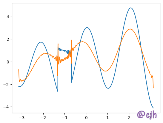
# 使用滤波器进行攻击
from scipy import signal

b, a = signal.butter(2, 0.8, 'lowpass')   #配置滤波器 8 表示滤波器的阶

# embed data
t = np.linspace(-np.pi, np.pi, 1024)
ar = (np.sin(t) + 3*np.cos(3*t)) * np.exp(0.1*t)
dst, diff = scale(ar, 100);
dst[30:40] = 1
ar_restore = inverse_scale(dst, diff)
plt.plot(t, ar_restore)

# attack
ar_restore = signal.filtfilt(b, a, ar_restore)
f = np.fft.fft(ar_restore)
f[3:80] = 0
f[-81:-3] = 0
ar_restore = np.fft.ifft(f).real
plt.plot(t, ar_restore)

# restore data
t_, _ = scale(t, 100)
dst, diff = scale(ar_restore, 100);
print(dst[30:40])

Summary

using the lossless scale algorithm can enhance the robustness of the watermark, but there still have a long way to go for practical use.